Estimating the Triage Line When There's No Baseline to Size It From

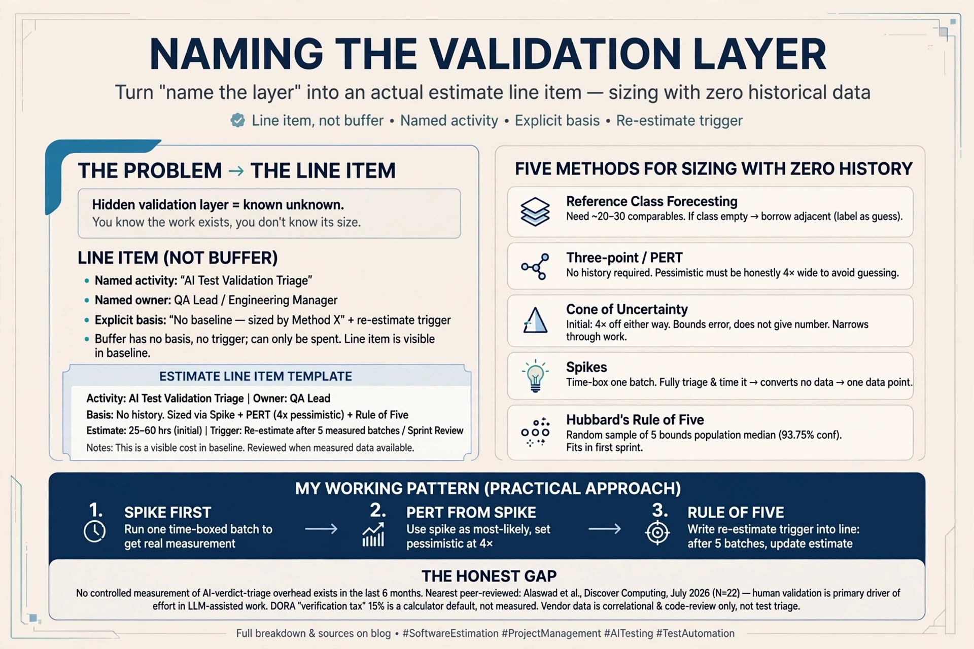
The last post (AI-Assisted Testing Adds a Validation Layer, It Doesn’t Remove One) ended on two open questions: what does “name the layer in the plan” look like as an actual line in the estimate — and how do you put a number on that line when nobody has measured it yet?

Short answer: the first question has a clean answer. The second doesn’t, and the honest move is to say so and pick the least-bad method.

Why the layer gets left out

Missing work in an estimate is rarely a math error. It’s an omission.

Steve McConnell’s Software Estimation (2006) has a section literally called “Omitted Activities.” The list of things estimates commonly leave out includes: attending change-control and triage meetings, answering testers’ questions, reviewing plans, estimates, code and test cases, learning new tools, and defect-tracking administration. (McConnell, Software Estimation (2006) — cited via secondary summary, section number not verified.)

Every item on that list is a form of validation overhead. AI-verdict triage is the same shape of work with a new name. It isn’t left out because it’s small — it’s left out because it’s between the activities people already know how to name.

McConnell’s later “17 Theses on Software Estimation” (2015) adds the reason it stays hidden: what gets called an “estimate” is very often a planning target or a commitment. (Thesis 10, stevemcconnell.com, 2015-08-02.) A target has pressure to be small. An omitted activity is the easiest way to keep it small without anyone lying.

Line item, not buffer

The instinct when you know a cost exists but can’t size it is to “add some padding.” That’s the wrong tool, and the estimation literature is fairly explicit about why.

• Padding is an undisclosed effort reserve. QSM’s guidance is that contingency should be visible, approved, and documented — not quietly folded into the numbers. (QSM, Zuber, 2012-04-19.)
• PMI’s contingency reserve is time or money for known risks that have an active response plan. It’s visible to everyone and can sit at the activity level. (PMI, PMBOK Guide — contingency reserve and management reserve definitions.)
• PMI’s management reserve is for unknown unknowns. It sits outside the baseline and is not the team’s to spend.

Triage of AI-generated tests is a known unknown: you know the work exists, you don’t know its size. By PMI’s own categories, that belongs inside the visible baseline — as a line, or at most as a named activity-level contingency — not in a management reserve and definitely not in silent padding.

What the line looks like in practice (my working format, not a standard):

Field	Example
Activity	Triage of AI-generated test results
Unit	per batch of generated tests (define “batch” — e.g. one generation run per module)
Owner	named person, not “the team”
Estimate	three-point: optimistic / likely / pessimistic (see below)
Basis	“no baseline — sized by method X, re-estimate after N measured batches”
Re-estimate trigger	after 5 measured batches, or when actuals leave the optimistic–pessimistic range

The last two rows are the whole point. A buffer has no basis field and no trigger. A line item that says “this is a guess, here is when it stops being a guess” can be challenged, tracked, and replaced. A buffer can only be spent.

Sizing with zero history: what the methods actually say

Now the hard part. Five standard approaches, and what each one offers when the reference data is empty.

1. Reference class forecasting — assumes the class exists

Kahneman and Lovallo’s 1993 paper distinguishes the inside view (reason about this specific case) from the outside view (treat it as one of a class and use the class statistics). Their finding: “decision makers have a strong tendency to consider problems as unique.” (Kahneman & Lovallo, Management Science, 1993, peer-reviewed.)

Flyvbjerg turned this into reference class forecasting: identify the reference class, establish its distribution, place your project in it. It works — but it wants roughly 20–30 comparable projects, and the choice of class dominates the answer (the “reference class problem”). (Reference class forecasting: Flyvbjerg, “From Nobel Prize to Project Management: Getting Risks Right,” Project Management Journal, 2006. The specific 20–30 figure comes from secondary summaries of his guidance and is not verified against a primary source — treat it as a rule of thumb, not a hard threshold.)

For AI-verdict triage the class is empty. Neither source gives guidance for that case. The best you can do is borrow an adjacent class (code review overhead, flaky-test triage, alert fatigue in ops) and state openly that you did. That’s an inside-view guess dressed as an outside view, and it should be labeled as one.

2. Three-point / PERT — doesn’t need history, needs honesty

The PERT formula from Malcolm et al. (1959): expected = (optimistic + 4 × likely + pessimistic) / 6, standard deviation = (pessimistic − optimistic) / 6. The three inputs come from experience or best guess; nothing in the method requires historical data.

The catch is the pessimistic value. With no baseline, the temptation is to set it “reasonably.” It has to be honestly wide, or the formula just launders one guess into three. For the rollout in the last post, an honest pessimistic value would have been “4× the optimistic,” which is roughly what happened.

3. Cone of Uncertainty — tells you how wrong, not what number

McConnell’s cone (2006, from earlier Boehm work) puts the initial estimate at up to 4× too high or 0.25× too low. Two things people miss about it:

• It’s a bound on error, not an estimate. It doesn’t give you the number; it tells you how much to distrust it.
• It narrows only through work that removes variability. Time passing doesn’t narrow it. Doing a spike does. (McConnell 2006; Construx; Jeff Atwood, Coding Horror, 2006.)

So the cone’s contribution to the zero-baseline case is: whatever line you write, write ±4× next to it, and schedule the work that shrinks that.

4. Spikes — buy a small baseline before committing

A spike (XP origin; Cohn’s Mountain Goat write-up, updated 2024) is a time-boxed research activity whose output is knowledge, not product — specifically knowledge that makes the next estimate better. The investment is fixed by the box.

Applied here: run one generation batch, triage it fully, time it. The spike costs one box. It converts “no data” into “one data point,” which is a different problem — see next.

5. Hubbard’s Rule of Five — the closest thing to a real answer

Douglas Hubbard (How to Measure Anything) states the Rule of Five: for any random sample of five from a population, there’s a 93.75% chance the population median lies between the smallest and largest of the five. His line: “If you know almost nothing, almost anything will tell you something.”

This is the one method that speaks directly to the empty-class case. Five measured triage batches bound the median triage time with 93.75% confidence. Five is small enough to do inside the first sprint of a rollout.

Caveats, so nobody over-reads it:

• The five need to be reasonably random, not the five easiest modules.
• It bounds the median, not the tail — and the tail is where the two months came from.
• It’s a bound, not a point estimate. The range from five batches can still be wide.

What I’d actually write in the estimate

Putting the five together, this is the pattern I’d use — opinion, not a standard:

1. Line item, not buffer. Named activity, named owner, explicit “no baseline” basis.
2. Spike first. One time-boxed batch, fully triaged and timed, before the estimate is committed.
3. PERT from the spike. Optimistic = spike result. Likely = 2× spike. Pessimistic = 4× spike (the cone’s outer bound). That’s a rule of thumb, not derived from data.
4. Rule of Five as the re-estimate trigger. After five measured batches, replace the PERT guess with the observed range. Write that trigger into the line.
5. Keep the basis visible. The line should say which of these steps produced the number, so the next person can tell a guess from a measurement.

Supporting evidence from 2026 — and its limits

Is validation effort actually the dominant cost, or is that just my one rollout? The 2026 sources point the same way, with caveats.

• Human validation dominates effort. Alaswad et al. (Discover Computing, 2026-07-06, peer-reviewed; 22 developers, 110 tasks, 3 LLMs) found that “human validation and corrective intervention emerge as the primary drivers of effort, outweighing artifact-level characteristics,” and that story points “fail to capture dominant sources of effort.” Adding human-intervention dimensions increased explained variance in effort “from approximately 72% to 80%” (per the abstract). Small N — the nearest peer-reviewed data point, not a definitive one.
• “Human Oversight Effort” as an estimation dimension. The same group’s earlier conceptual paper (Frontiers in AI, 2026-03-23, peer-reviewed) names reviewing, validating, testing and correcting LLM output as a core dimension of estimation. Conceptual only — the authors state the framework “has not yet been empirically calibrated on large industrial datasets.”
• DORA’s “verification tax.” Secondary write-ups (InfoQ, zenn) of DORA’s ROI of AI-assisted Software Development report describe it naming a “verification tax” as one of three causes of the productivity dip that follows AI adoption, and its sample ROI calculator using a default assumption of a 15% productivity drop over 3 months. Caveat: the primary report is a gated PDF; the phrase, the “three causes,” the version/date, and the 15%/3-month figure are taken from those secondary sources and were not independently verified against DORA’s own text. Even if accurate, that 15% is an input someone typed into a calculator, not a measured result — don’t quote it as data.
• Review load goes up. Two vendor telemetry reports point at more review work per PR: Faros AI (blog, 2026-05-21, drawing on its AI Engineering Report 2026 dataset — sample size for these specific figures not independently confirmed) reports median time in PR review up 441.5% and bugs per PR up 54%; LinearB (2026-05-04; 8.1M PRs, ~4,800 teams) reports AI-assisted PRs about 2.5× larger at the 75th percentile with pickup wait more than 5× longer. Both are correlational, neither has a control group, Faros doesn’t state how “AI-assisted” was attributed, and both measure general code review — not test-verdict triage. Directional support only.

The gap, stated plainly: no controlled measurement of AI-verdict-triage overhead exists within the last six months. And no source, classic or 2026, solves reference class forecasting for a genuinely empty class. The methods above don’t fill that gap. They make the guess visible, bounded, and replaceable — which is the most an estimate can honestly do until the data exists.

Where this goes next

• Processes / estimation — autonomous AI runs estimate like Waterfall, not Agile: an agent that generates 400 tests in one run delivers a batch, not an increment — the validation can’t be spread across sprints, it lands all at once and has to be sized up front. The angle: contrast the story-point/velocity assumptions (continuous flow, effort scales with artifact size) against the batch shape of AI output, using Alaswad’s “story points fail to capture dominant sources of effort” finding as the pivot. Written up: A Batch Is Not an Increment.